Table Of Content

Then these 15 linear combinations or contrasts are also normally distributed with some variance. If we assume that none of these effects are significant, the null hypothesis for all of the terms in the model, then we simply have 15 normal random variables, and we will do a normal random variable plot for these. We get a normal probability plot, not of the residuals, not of the original observations but of the effects.
Lesson 6: The \(2^k\) Factorial Design
When 40 year olds, however, are given a 5 mg pill or a 10 mg pill, 15% suffer from seizures at both of these dosages. There is an increasing chance of suffering from a seizure at higher doses for 20 year olds, but no difference in suffering from seizures for 40 year olds. Thus, there must be an interaction effect between the dosage of CureAll, and the age of the patient taking the drug. When you have an interaction effect it is impossible to describe your results accurately without mentioning both factors. You can always spot an interaction in the graphs because when there are lines that are not parallel an interaction is present. If you observe the main effect graphs above, you will notice that all of the lines within a graph are parallel.
Building Fractional Factorials: a Methodology for Symmetric and Asymmetric Designs
This arises, in part, from the fact that the effects of any given factor are defined by its average over the levels of the other factors in the experiment. It is important, therefore, for researchers to interpret the effects of a factorial experiment with regard to the context of the other experimental factors, their levels and effects. This does not reflect any sort of problem inherent in factorial designs; rather, it reflects the trade-offs to consider when designing factorial experiments.
A catalogue of three-level regular fractional factorial designs
Factor's new Ostro VAM blurs boundaries with aero and lightweight design - GCN - Global Cycling Network
Factor's new Ostro VAM blurs boundaries with aero and lightweight design.
Posted: Wed, 14 Feb 2024 08:00:00 GMT [source]
None of the levels were specified as they appear as -1 and 1 for low and high levels, respectively. The following Yates algorithm table was constructed using the data from the interaction effects section. Since the main total factorial effect for AB is non-zero, there are interaction effects. This means that it is impossible to correlate the results with either one factor or another; both factors must be taken into account. The following Yates algorithm table using the data from second two graphs of the main effects section was constructed.
The figure below contains the DOE table of trials including the two responses. Ignoring the first row, look in the last stage and find the variable that has the largest relative number, then that row indicates the MAIN TOTAL EFFECT. The Main Total Effect can be related to input variables by moving along the row and looking at the first column.
Let's use the dataset (Ex6-2.csv) and work at finding a model for this data with Minitab... In the example that was shown above, we did not randomize the runs but kept them in standard order for the purpose of seeing more clearly the order of the runs. In practice, you would want to randomize the order of run when you are designing the experiment. In the example above the A, B and C each are defined by a contrast of the data observation totals. Therefore you can define the contrast AB as the product of the A and B contrasts, the contrast AC by the product of the A and C contrasts, and so forth. One nice feature of the Yates notation is that every column has an equal number of pluses and minuses so these columns are contrasts of the observations.
& 4. Measure Performance to Find an Effect
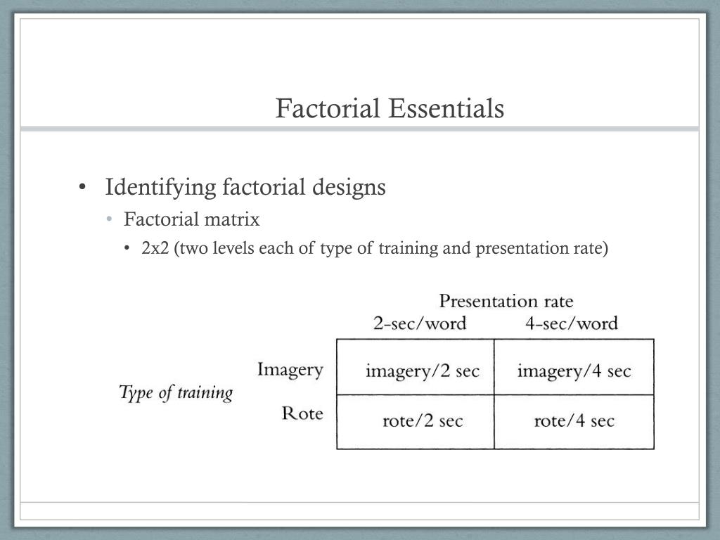
Under this assumption, estimates of such high order interactions are estimates of an exact zero, thus really an estimate of experimental error. If these values represent "low" and "high" settings of a treatment, then it is natural to have 1 represent "high", whether using 0 and 1 or −1 and 1. This is illustrated in the accompanying table for a 2×2 experiment. This can be conducted with or without replication, depending on its intended purpose and available resources. It will provide the effects of the three independent variables on the dependent variable and possible interactions. The number of digits tells you how many independent variables (IVs) there are in an experiment, while the value of each number tells you how many levels there are for each independent variable.
Examples of Factorial Designs
Thus far we have seen that factorial experiments can include manipulated independent variables or a combination of manipulated and non-manipulated independent variables. But factorial designs can also include only non-manipulated independent variables, in which case they are no longer experiments but are instead non-experimental in nature. This can be conceptualized as a 2 × 2 factorial design with mood (positive vs. negative) and self-esteem (high vs. low) as non-manipulated between-subjects factors. But factorial designs can also include only non-manipulated independent variables, in which case they are no longer experiment designs, but are instead non-experimental in nature. But factorial designs can also include only non-manipulated independent variables, in which case they are no longer experiments but are instead non-experimental (cross-sectional) in nature.
Types of Factorial Designs
In an RCT an “active” treatment arm or condition is statistically contrasted with a “control” treatment arm or condition (Friedman, Furberg, & Demets, 2010). The two conditions should be identical except that the control condition lacks one or more ICs or features that are provided to the active condition. The random assignment of participants to the treatment arms means that the two groups of assigned participants should differ systematically only with regard to exposure to those features that are intentionally withheld from the controls. In smoking cessation research a common RCT design is one in which participants are randomly assigned to either an active pharmacotherapy or to placebo, with both groups also receiving the same counseling intervention. The red bars show the conditions where people wear hats, and the green bars show the conditions where people do not wear hats. For both levels of the wearing shoes variable, the red bars are higher than the green bars.
And the individual terms, B, C, D, BC and BD, are all significant, just as shown on the normal probability plot above. Notice also the use of the Yates notation here that labels the treatment combinations where the high level for each factor is involved. If only A is high then that combination is labeled with the small letter a. You would find these types of designs used where k is very large or the process, for instance, is very expensive or takes a long time to run. In these cases, for the purpose of saving time or money, we want to run a screening experiment with as few observations as possible. When we introduced this topic we wouldn't have dreamed of running an experiment with only one observation.
Or it could be that people who are lower in SES tend to come from certain ethnic groups that emphasize generosity more than other ethnic groups. The researchers dealt with these potential third variables, however, by measuring them and including them in their statistical analyses. They found that neither religiosity nor ethnicity was correlated with generosity and were therefore able to rule them out as third variables. This does not prove that SES causes greater generosity because there could still be other third variables that the researchers did not measure. But by ruling out some of the most plausible third variables, the researchers made a stronger case for SES as the cause of the greater generosity.
You have to be careful about using the mean in one case, and the media in another ... For those of you who have studied heteroscedastic variance patterns in regression models you should be thinking about possible transformations. There is a gap in the histogram of other residuals but it doesn't seem to be a big problem.


No comments:
Post a Comment